Views

The grid.view method returns a copy of a dataset cropped to the grid’s current view. The grid’s current view is defined by its viewfinder attribute, which contains five properties that fully define the spatial reference system:

• affine: An affine transformation matrix.
• shape: The desired shape (rows, columns).
• crs : The coordinate reference system.
• mask : A boolean array indicating which cells are masked.
• nodata : A sentinel value indicating ‘no data’.

Initializing the grid view

The grid’s view will be populated automatically upon reading the first dataset.

grid = Grid.from_raster('./data/dem.tif')

grid.affine

Output...

Affine(0.0008333333333333, 0.0, -97.4849999999961,
       0.0, -0.0008333333333333, 32.82166666666536)

grid.crs

Output...

Proj('+proj=longlat +datum=WGS84 +no_defs', preserve_units=True)

grid.shape

Output...

(359, 367)

grid.mask

Output...

array([[ True,  True,  True, ...,  True,  True,  True],
       [ True,  True,  True, ...,  True,  True,  True],
       [ True,  True,  True, ...,  True,  True,  True],
       ...,
       [ True,  True,  True, ...,  True,  True,  True],
       [ True,  True,  True, ...,  True,  True,  True],
       [ True,  True,  True, ...,  True,  True,  True]])

We can verify that the spatial reference system is the same as that of the originating dataset:

dem = grid.read_raster('./data/dem.tif')

grid.affine == dem.affine

Output...

True

grid.crs == dem.crs

Output...

True

grid.shape == dem.shape

Output...

True

(grid.mask == dem.mask).all()

Output...

True

Viewing datasets

First, let’s delineate a watershed and use the grid.view method to get the results.

# Resolve flats
inflated_dem = grid.resolve_flats(dem)

# Compute flow directions
fdir = grid.flowdir(inflated_dem)

# Specify pour point
x, y = -97.294167, 32.73750

# Delineate the catchment
catch = grid.catchment(x=x, y=y, fdir=fdir, xytype='coordinate')

# Get the current view and plot
catch_view = grid.view(catch)

Plotting code...

fig, ax = plt.subplots(figsize=(8,6))
fig.patch.set_alpha(0)
plt.imshow(catch_view, cmap='Greys_r', zorder=1)
plt.title('Catchment', size=14)
plt.tight_layout()

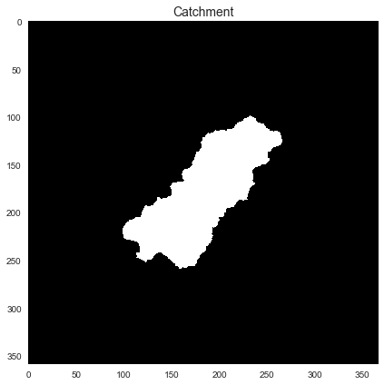
Note that in this case, the original raster and its view are the same:

(catch == catch_view).all()

Output...

True

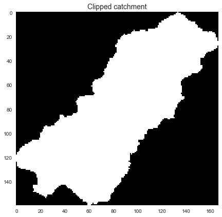
Clipping the view to a dataset

The grid.clip_to method clips the grid’s current view to nonzero elements in a given dataset. This is especially useful for clipping the view to an irregular feature like a delineated watershed.

# Clip the grid's view to the catchment dataset
grid.clip_to(catch)

# Get the current view and plot
catch_view = grid.view(catch)

Plotting code...

fig, ax = plt.subplots(figsize=(8,6))
fig.patch.set_alpha(0)
plt.imshow(catch_view, cmap='Greys_r', zorder=1)
plt.title('Clipped catchment', size=14)
plt.tight_layout()

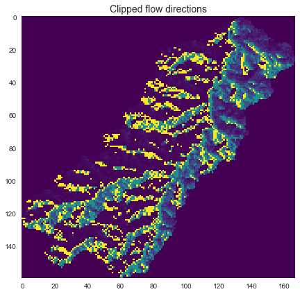
We can also now use the view method to view other datasets within the current catchment boundaries:

# Get the current view of flow directions
fdir_view = grid.view(fdir)

Plotting code...

fig, ax = plt.subplots(figsize=(8,6))
fig.patch.set_alpha(0)
plt.imshow(fdir_view, cmap='viridis', zorder=1)
plt.title('Clipped flow directions', size=14)
plt.tight_layout()

Tweaking the view using keyword arguments

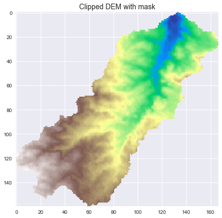
Setting the “no data” value

The “no data” value in the output array can be specified using the nodata keyword argument. This is often useful for visualization.

dem_view = grid.view(dem, nodata=np.nan)

Plotting code...

fig, ax = plt.subplots(figsize=(8,6))
fig.patch.set_alpha(0)
plt.imshow(dem_view, cmap='terrain', zorder=1)
plt.title('Clipped DEM with mask', size=14)
plt.tight_layout()

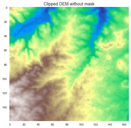
Toggling the mask

The mask can be turned off by setting apply_output_mask=False.

dem_view = grid.view(dem, nodata=np.nan,
                     apply_output_mask=False)

Plotting code...

fig, ax = plt.subplots(figsize=(8,6))
fig.patch.set_alpha(0)
plt.imshow(dem_view, cmap='terrain', zorder=1)
plt.title('Clipped DEM without mask', size=14)
plt.tight_layout()

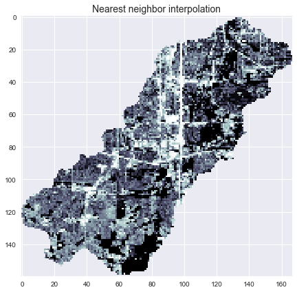
Setting the interpolation method

By default, the view method uses a nearest neighbors approach for interpolation. However, this can be changed using the interpolation keyword argument.

# Load a dataset with a different spatial reference system
terrain = grid.read_raster('./data/impervious_area.tiff', window=grid.bbox,
                           window_crs=grid.crs)

Nearest neighbor interpolation

# View the new dataset with nearest neighbor interpolation
nn_interpolation = grid.view(terrain, nodata=np.nan)

Plotting code...

fig, ax = plt.subplots(figsize=(8,6))
fig.patch.set_alpha(0)
plt.imshow(nn_interpolation, cmap='bone', zorder=1)
plt.title('Nearest neighbor interpolation', size=14)
plt.tight_layout()

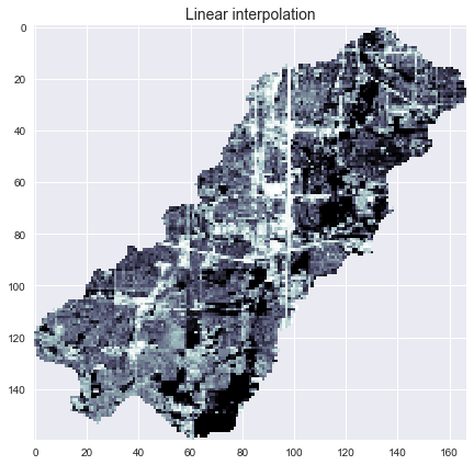
Linear interpolation

# View the new dataset with linear interpolation
lin_interpolation = grid.view(terrain, nodata=np.nan, interpolation='linear')

Plotting code...

fig, ax = plt.subplots(figsize=(8,6))
fig.patch.set_alpha(0)
plt.imshow(lin_interpolation, cmap='bone', zorder=1)
plt.title('Linear interpolation', size=14)
plt.tight_layout()

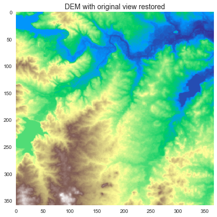
Setting the view manually

The grid.viewfinder attribute can also be set manually.

# Reset the view to the dataset's original view
grid.viewfinder = dem.viewfinder

# Plot the new view
dem_view = grid.view(dem)

Plotting code...

fig, ax = plt.subplots(figsize=(8,6))
fig.patch.set_alpha(0)
plt.imshow(dem_view, cmap='terrain', zorder=1)
plt.title('DEM with original view restored', size=14)
plt.tight_layout()